Investigating the Temperature Dependence of the Speed
of Sound
Lanqiao George Yuan
UBC Department of Physics and Astronomy
georgeyuan15@hotmail.com
Motivated by the observation that the intonation of musical instruments is affected by temperature changes, I set out to investigate the temperature dependent properties of sound. In particular, I discovered that the speed of sound is proportional to the temperature of its medium.
This website is split into two sections:
- The theory of sound propagation. Here we learn how sound waves are modeled in physics, and derive an expression for the speed of sound.
- The experiment. This section describes my experiment to measure the temperature dependence of the speed of sound. We also discuss the experimental results and relate them back to theory.
Also included is a PowerPoint presentation of my project, which I presented to two physics 12 classes at University Hill Secondary School.
The Theory of Sound
We
all know what sound is intuitively, but what is the physical basis of a sound
wave?
Sound is a longitudinal travelling wave caused by an oscillation of pressure (the compression and dilation of particles) in matter.
The following animation illustrates how particles mediate a sound wave. Notice that each specific particle is merely moving back and forth – the travelling wave is merely a long-range pattern in the particle oscillations.
http://paws.kettering.edu/~drussell/Demos/waves/wavemotion.html
Some other names for sound waves are pressure waves, compression waves, and density wave; these names derive from the motion of particles that carry sound.
So how do we relate the physical picture of sound to what we hear?
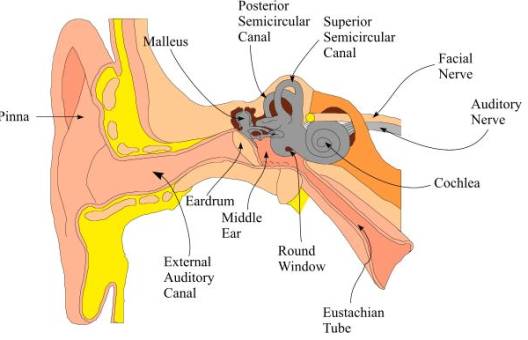

This is a somewhat complicated diagram of all the structures in the ear, but the only information we require from it are the eardrum and auditory nerve.
The eardrum is a thin membrane near the outer ear. Pressure waves in the air hit the eardrum and cause it to oscillate in an identical pattern. The eardrum’s vibration information is transferred through various inner ear structures, eventually reaching the brain through the auditory nerve. (I highly encourage you to look up for yourself how the inner ear works – it is a fascinating topic!) In any case, the brain interprets this information from the eardrums as sound.
Different patterns of vibration of course correspond to different sound. Some of the properties of sound are:
(1) Pitch – this is determined by the frequency of the eardrum’s vibrations. Higher frequencies correspond to higher pitches, and lower frequencies to lower pitches. The normal range of human hearing is 20 Hz to 20 kHz.
(2) Volume – this is determined by the amplitude (displacement from neutral position) of the eardrum’s vibrations. Larger displacements correspond to louder sounds, and smaller displacements correspond to softer sounds. Sound volume is measured on a logarithmic scale called the Decibel Scale.
(3) Speed – how fast does a sound wave travel in air, and what factors affect its speed? This is the property that we will investigate in our experiment.
Now that we know what sound is, how do we model sound mathematically?
Sound is somewhat tricky to describe because it is an abstract concept. A sound wave isn’t an object with definite boundaries or position; it’s a type of particle motion – the travelling compressions and rarefactions in a medium.
The most conceptually straight-forward way to describe sound is to simply keep track of the positions of every particle that mediates the sound wave. Simple, right? Well not quite. The number of particles in a normal acoustic system exceeds 1023 (Avogadro’s number)! It is impossible to calculate the position of every single particle.
The real method uses the exact same idea. However, instead of keeping track of every particle individually, we use probability and statistics to “guess” the collective behaviour of the particles. The branch of physics that uses statistics to model systems with extremely large number of components is called statistical mechanics, sometimes referred to as thermodynamics. Sound is a statistical mechanical phenomenon.
Before delving into a statistical mechanical description of sound, we first need some important definitions:
(1) Bulk modulus (K)
The bulk modulus is a measure of the elasticity of a gas; in order words, it describes how easily a gas can be compressed.
It is defined as ![]() , where V is the
gas volume and P is the gas pressure.
Δ of course means “change in.”
, where V is the
gas volume and P is the gas pressure.
Δ of course means “change in.”
Rearranging this
expression gives ![]() , and here we can easily see that K is completely analogous to the spring constant k in Hooke’s law
, and here we can easily see that K is completely analogous to the spring constant k in Hooke’s law ![]() .
.
In Hooke’s law, to stretch or compress a spring by a distance Δx requires a force proportional to the spring constant k. A higher spring constant means that a larger force is needed for the same displacement Δx, so a higher spring constant means a stiffer spring.
Likewise, to compress a gas by a relative volume ΔV/V, a pressure proportional to the bulk modulus K is required. Higher K corresponds to a less compressible gas. The relative volume change is used rather than absolute volume change because unlike solid springs, gases expand to fill their container – a 1L change in a 100L container is small; a 1L change in a 2L container is huge.
For diatomic
gases ![]() .
.
Diatomic gases contain 2 atoms per molecule; Nitrogen is an example of a diatomic gas. For these types of gases, the bulk modulus is dependent on the gas pressure and a constant γ called the adiabatic index, explained below.
(2) Adiabatic process
An adiabatic process is a physical process in which heat does not enter or leave the system. The compression and dilation of air to form a sound wave is an adiabatic process, because the thermal energy associated with compression dissipates much slower than the speed of the sound wave.
(3) Adiabatic index (γ)
Formally, γ is defined to be the ratio of the specific heat capacity of a substance at constant pressure (CP) to its specific heat capacity at constant volume (CV). Clearly this definition is far beyond our needs; for our purposes, we can think of γ simply as a constant in the expression for K necessary to take into account the thermal energy associated with gas compression, which adds to the gas pressure.
Now we had all the tools we need to derive
an expression for the speed of sound. Sort of. A rigorous derivation of the
speed of sound from first principles in statistical mechanics is possible, but
extremely mathematically complex. Instead, we shall start midway with a more
easily accessible equation ![]() , where c is the
speed of sound, ρ is the gas
density, and K is of course the bulk
modulus.
, where c is the
speed of sound, ρ is the gas
density, and K is of course the bulk
modulus.
Try this as a rudimentary justification of the above formula:
(1) Find 2 large springs, one stiff (high spring constant) and one springy (low spring constant).
(2) Drop a weight on each spring. You should see the spring with the lower spring constant take more time to compress and expand, whereas the weight would bounce much faster off the stiffer spring.
(3) The situation is analogous to compression waves in gas – a “stiffer” gas (one with a higher bulk modulus) will transfer compressions faster, whereas a more compressible gas will take time to compress and rarefy. Therefore, the speed of sound is proportional to K. The square root dependence is of course more difficult to justify, so you’ll just have to trust me.
There is no simple demonstration for the density term; but intuitively, it makes sense that it is harder to send compression waves through a denser medium; therefore c is inversely proportional to ρ.
Anyways, going back to the derivation: ![]() .
.
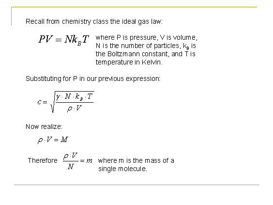
So far we don’t see any dependence on temperature. However, recall that gases are (ideally) governed by the ideal gas law, which relates gas pressure to gas temperature. Essentially, since c is dependent on P and P is dependent on T, c is then dependent on T.
(From this point, I feel my original PowerPoint slides are sufficiently detailed to be copied and pasted to finish the derivation.)
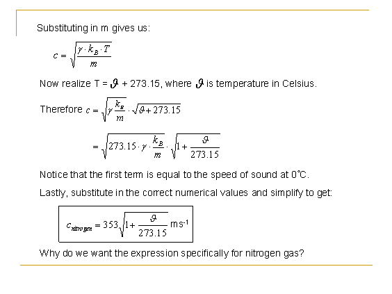
And the answer to the above question on the slide: Because in the experiment, we will be using liquid nitrogen to control the temperature of the sound wave. This will become clear in the experiment design section.
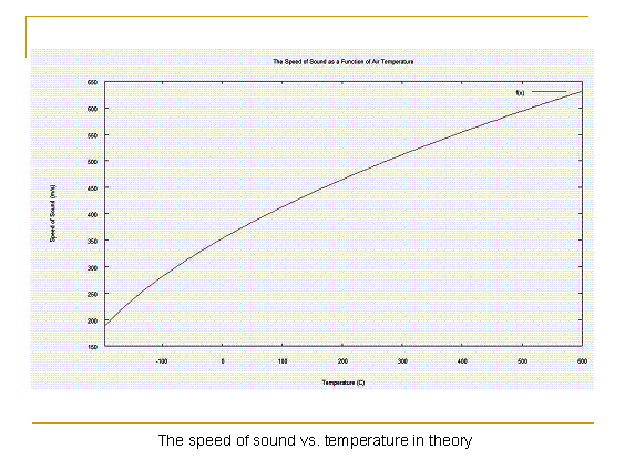
In any case, graphing the above function gives us:
Experiment design
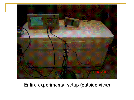
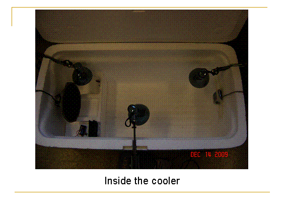
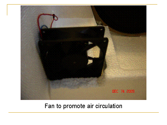
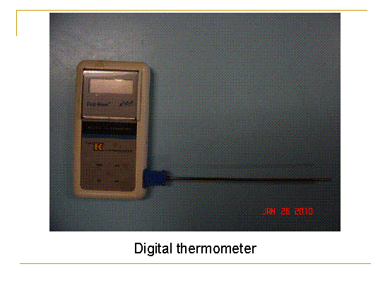
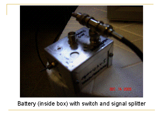
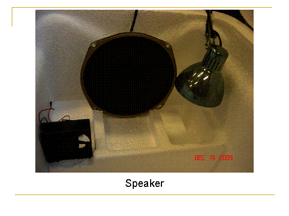
List of apparatus:
(1) Large Styrofoam cooler
(2) Liquid nitrogen
(3) Heating lamps (60W)
(4) Digital thermometer
(5) Electric fan
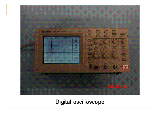
(6) Two-channel digital oscilloscope
(7) Speaker
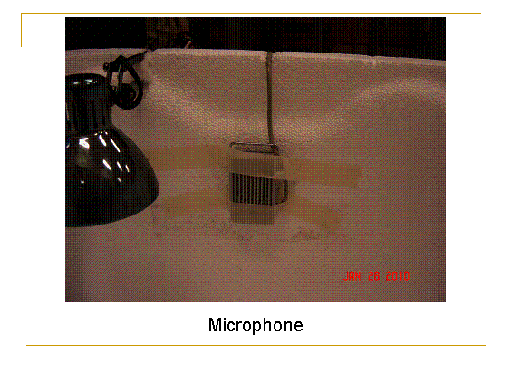
(8) Microphone
(9) Battery (9V) with switch
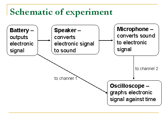
(1) Battery outputs an electronic signal, which is split between the speaker and channel 1 of the oscilloscope.
(2) Electricity travels almost instantaneously through wires.
(3) The speaker changes the electronic signal from the battery into an acoustic signal (sound).
(4) The sound wave travels through the length of the cooler before reaching the microphone. Along this leg of the trip to the oscilloscope, the signal speed is NOT instantaneous; it is the speed of sound.
(5) The microphone converts the acoustic signal back into an electric signal, which then travels to channel 2 of the oscilloscope.
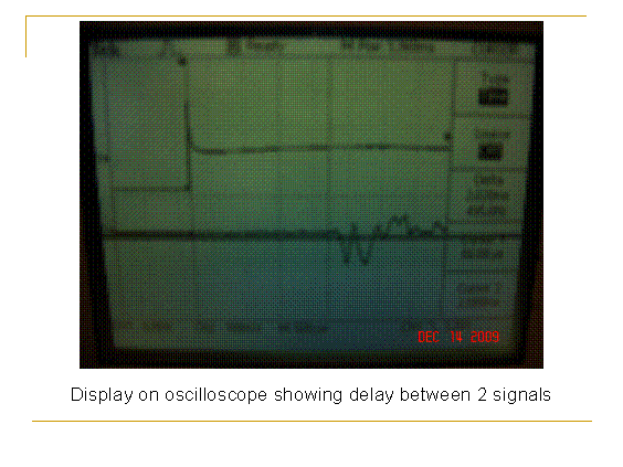
(6) There will be a time delay between the channel 1 and channel 2 signals – this time corresponds to the time it took for sound to travel from the speaker to the microphone.
(7) By dividing the distance between the speaker and the microphone by the time delay, we get the speed of sound.
(8) We use liquid nitrogen and heating lamps to control the temperature inside the cooler. Repeating this procedure at different temperatures will measure the temperature dependence of the speed of sound.
Photos
of the experimental setup


The
process of taking a data point
(1) Pour liquid nitrogen into the cooler – the temperature should settle down to –60˚C.
(2) Turn on battery to send a voltage pulse.
(3) This pulse triggers the oscilloscope to (1) start reading and (2) freeze graph on screen (pre-set oscilloscope functions).
(4) Immediately record the temperature.
(5) Use oscilloscope cursors to measure the time delay between the signals on channels 1 and 2.
(6) Switch on the heating lamps – the temperature in the cooler will steadily rise.
(7) Repeat steps 2 – 6 at higher and higher temperatures.
Data
analysis and results
Our raw gives us, at each temperature, the travel time Δt of the sound wave. To extract the speed of the wave at each temperature, we simply need to divide the distance between the speaker and microphone by each Δt. That distance has been measured to be 73 cm.
Now we can graph the speed of sound against temperature and see how closely our data matches up with theoretical predictions. The program I used to generate these graphs is Gnuplot, but any program that can plot functions and individual data points will do the same job.

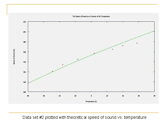
While the data points do not perfectly match up with theory, the general trend that the speed of sound rises with temperature is clear. There are many sources of uncertainty in this experiment which all contribute to the less than perfect results:
(1) The distance between speaker and microphone is not exact.
(2) Temperature distribution inside cooler may not be completely uniform.
(3) Air may leak out of cooler – escaping nitrogen replaced by normal air. Recall that for the speed of sound is different in different gases.
(4) Oscilloscope screen does not clearly define the beginning of the microphone signal. This is due to (i) acoustic noise from sounds inside room, (ii) electronic noise from battery, microphone, etc., and (iii) simply a less than perfect display and cursor system – we are measuring Δt by eye after all.
Furthermore, the theory itself is not
exact, because we made some approximations (![]() and
and ![]() ) in the derivation. So we are essentially comparing
inaccurate experimental data to an approximate theory. I’m surprised too that
the results are decent!
) in the derivation. So we are essentially comparing
inaccurate experimental data to an approximate theory. I’m surprised too that
the results are decent!
Anyways, in summary:
- What we perceive as sound is actually oscillations of air particles; these oscillations are caused by pressure waves travelling through the air.
- Sound waves are mathematically described by statistical mechanics.
- The speed of sound is dependent on the temperature of the medium carrying it, and obeys the equation:
![]()