Materials List
-
Paracord 6+meters long
This project used this one from amazon.ca -
A 5-pin bowling ball with a hook on it
A screw-hook from the hardware store and a drill should work if there are no ready made bobs on hand. -
Two glass funnels
This project used a TLG 50mm and a TLG 65mm funnel. Anything in that size range should work though. What’s important is that the funnels be glass -- plastic funnels have too much friction for a smooth sand flow. -
Art Sand
This project used this one from Micheals. -
A Door-Frame Pull-Up Bar
This project used this one from amazon.ca .
-
Duct Tape
-
A Plastic Water Bottle
One of the funnels needs to fit snugly inside. This project used a bottle from Glaceau smartwater. -
Hot-Glue + Gun
-
A Measuring Tape
-
Paper
Large sheets or a roll is best. -
Washi Tape
(optional) -
A Broom.
(optional)
Steps


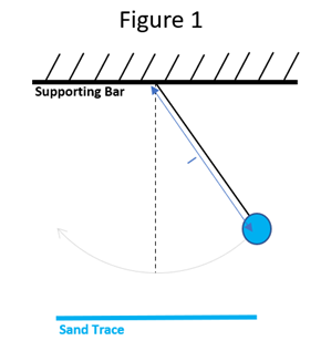
The position of the bob of a pendulum swinging back and forth in
a
plane as illustrated in Figure 1 can be expressed as![]() ) where
x
is the horizontal position of the bob, t is time,
) where
x
is the horizontal position of the bob, t is time, ![]() , is the
angular
frequency,
, is the
angular
frequency, ![]() is the
phase and A is the amplitude. However, if you imagine the pendulum dropping
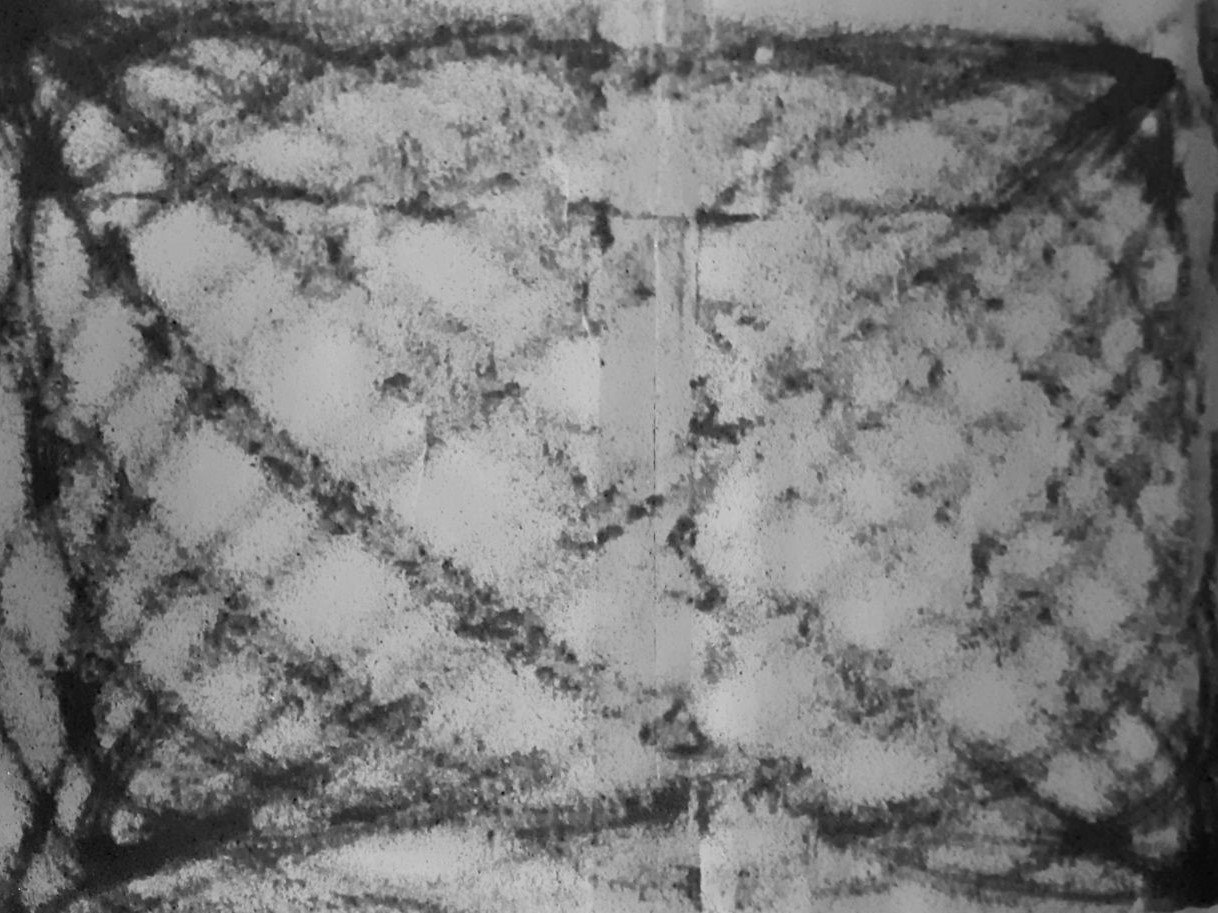
sand as it swings, you will see nothing more than a single line of sand on the floor
under the plane in which the bob goes back and forth. In order to see the sinusoidal
behavior, you would need to be able to distinguish sand that fell at one time from
sand
that fell at a different time when the bob was in the same place. That could be
achieved
by putting a paper on the floor and slowly pulling it at a constant speed. But
another
way of seeing a time dependent trace is if the pendulum is not limited to swinging
in a
plane, but instead, is allowed to swing in both directions. In this case, the motion
in
each orthogonal direction must be sinusoidal as the resulting more complex motion
can be
seen as a superposition of two perpendicular planar swings. The equations of motion
of
this 2D pendulum are as follows:
is the
phase and A is the amplitude. However, if you imagine the pendulum dropping
sand as it swings, you will see nothing more than a single line of sand on the floor
under the plane in which the bob goes back and forth. In order to see the sinusoidal
behavior, you would need to be able to distinguish sand that fell at one time from
sand
that fell at a different time when the bob was in the same place. That could be
achieved
by putting a paper on the floor and slowly pulling it at a constant speed. But
another
way of seeing a time dependent trace is if the pendulum is not limited to swinging
in a
plane, but instead, is allowed to swing in both directions. In this case, the motion
in
each orthogonal direction must be sinusoidal as the resulting more complex motion
can be
seen as a superposition of two perpendicular planar swings. The equations of motion
of
this 2D pendulum are as follows:
![]()
![]() .
.
These parametric equations form a 2-dimensional curve which the sand will trance out
as
the pendulum swings. The period, T, for each planar swing is, ![]() , where
g
is the gravitational constant, and l is the radius of rotation of the swing
(the string length for the pendulum in Figure 1). The angular frequency is then
, where
g
is the gravitational constant, and l is the radius of rotation of the swing
(the string length for the pendulum in Figure 1). The angular frequency is then ![]() , and so
we see
that for a simple pendulum hanging from a single string (as in Figure 1) the
period/frequency must be the same for motion in both the x and y
directions. This restricts the shapes the sand can trace out to being ellipses.
, and so
we see
that for a simple pendulum hanging from a single string (as in Figure 1) the
period/frequency must be the same for motion in both the x and y
directions. This restricts the shapes the sand can trace out to being ellipses.
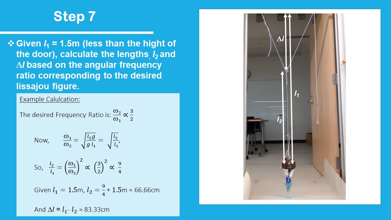
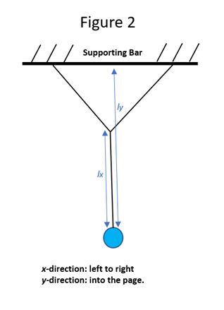
Now, the pendulum in this demonstration is the pendulum in Figure 2, which does not
have
the same radius of rotation for swings in the x plan as in the y
plane. For swings in the x-direction the radius of rotation,
lx in Figure 2, is the length of the bottom string, from
the
bob to the intersection of the Y shaped structure. On the other hand, when the
pendulum
is swung in the y-direction, the radius of rotation, ly
in
Figure 2, is the vertical distance from the bob to the top of the Y, or the bar from
which the pendulum is hung. Thus, this pendulum can have different periods and
angular
frequencies in the two directions and so, depending on the exact period in each
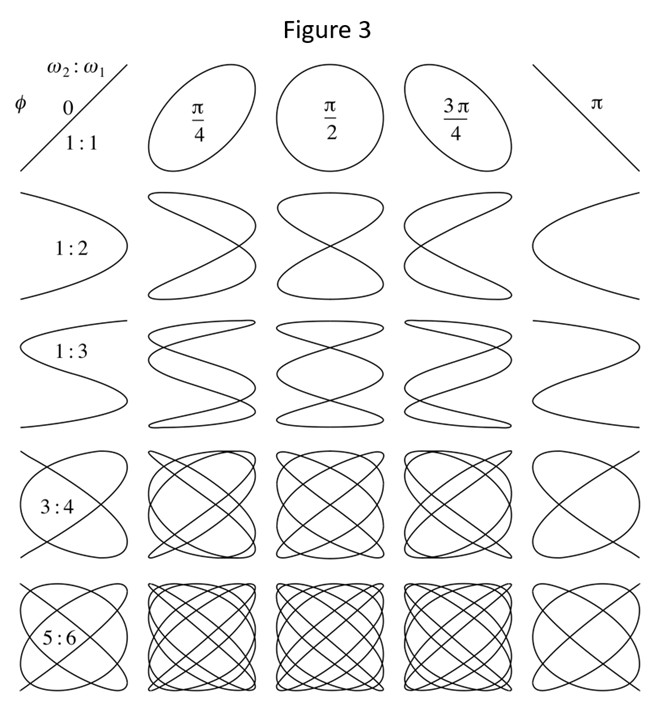
direction, it can make a whole set of looped figures called Lissajous figures after
the
19th century French physicist Jules Lissajous. The Lissajous table
(Figure 3)
shows how the shapes change based on the ratio of ![]() and
and ![]() , the
angular frequencies in the x and y
directions respectively.
, the
angular frequencies in the x and y
directions respectively.
Lesson Overview
This activity is designed for a Physics 11 or 12 classroom in British Columbia, Canada.
All the documents used for the presentation can be downloaded here:
- the slides,
- the blank worksheet,
- the worksheet solution,
- and the spreadsheet used to demonstrate the relationship between string length and period.
It is also useful to have a bob on a string other than the one built into the 3D pendulum to use for explanations (a 2nd bowling ball was used in this demonstration but even a simple rock tied to a string is fine).
The flow of the lesson can be broken into 5 parts which are outlined below along with some of the approaches used in this demo.
Introductory remarks:
- Lissajous-like figures are being used to produce real art on the market. These range from digital images to mechanically painted canvases.
- Review of a 2D pendulum:
Students will be encouraged to contribute as much as possible to this so it will serve as a warmup exercise. It will also serve as a brief assessment of where the class is at for the person running the activity.
- Key points to cover:
- Force diagram for the pendulum (have students give you suggestions before moving to the slide with the completed diagram).
- What does the projected trajectory look like? This can be targeted first by swinging a simple string+bob pendulum in my hand as asking what it would trance on the floor: a line.
- Present the equation of motion and the meaning of its parameters (note deriving the equation is beyond the scope of this lesson though it could be done with a more advanced class). It may be good to point out the difference and relationship between the sinusoidal equation and the linear projection of the trajectory.
- Once familiar with the different parameters, what physical variables does the period/frequency of the swings depend on? It depends on length (but not on mass !!).
- In order to convince students of the validity of the formula given for the period as a function of string length, the pre-prepared spreadsheet can be used. It has plot with period on the y-axis and string length on the x-axis. The blue line in the plot is the model, and there are a couple of points where the period has been measures. Students should be asked to pick a string length and time the period of the pendulum after adjusting it to that length, thus allowing them to add a point to the spreadsheet and insure it falls on the model. In order to get accurate enough measurements, it is necessary to time 10+ full-cycles swings and divide the time by the number of swings. Simply adding the new data to columns E and F is enough to have them show up on the chart.
- Check understanding by asking how one should change the string length if one wants to make the period/frequency go up/down.
- Adding a dimension:
Assign directions for x and y axes relative to the classroom walls, then swing the bob on a string used above for measuring the period, in the y=0 plane. This will give the sinusoidal trajectory x(t) discussed in part 1. Then, rotate, and swing the bob in the x=0 plane. Ask what the trajectory is now. Since the choice of coordinate system doesn’t affect the motion, one concludes that it must be the same function but with y in the place of x. Finally swing the pendulum in a circle or other 2d figure. Ask again about the trajectory. You’ll likely hear “complicated” or the equivalent in blank stares. At this point it may be helpful to do a little Socratic questioning along the lines of “Yes, but… Does motion in one direction affect the motion in the other direction? What is the x component of the trajectory? What is the y component?”.
- Key points to get across:
- X and Y components of the trajectories must have the same sinusoidal form.
- Frequencies cannot be different for a single string length. However, they can be different if the string length/radius of rotation is different in the two directions.
- There may be a phase difference (optional depending how quickly students get frequencies in the above point…).
- Parametric Trajectories and Lissajous Figures:
This part of the lesson starts with Part 1 of the worksheet which has students connect to Geogebra’s online parametric grapher and plot some trajectories. The first questions lead students to discover the importance of the frequency ratio to the shape of the trajectory, and the 2nd page has students fill in a Lissajous table, a table of different trajectories based on frequency ratio and phase (see worksheet solution).
- Tips:
- Take a few minutes to explain what parametric equations are, if students haven’t seen it, or haven’t seen it in a while, it will save a lot of time on the worksheet.
- Insist that students get out their laptops as the graphing tool often doesn’t display correctly on phones. Students that try on their phone first will waste a lot of time.
- If students are struggling to complete the table in a reasonable time ask them to only complete the leftmost column (where there is no phase difference).
At the end of the time for the first part of the worksheet have a brief full class discussion/sharing of results to make sure the entire class has developed an understanding of the impact of frequency on trajectory shape.
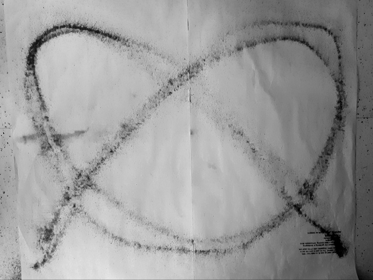
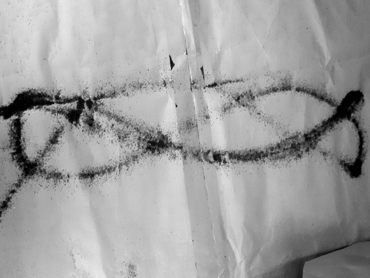
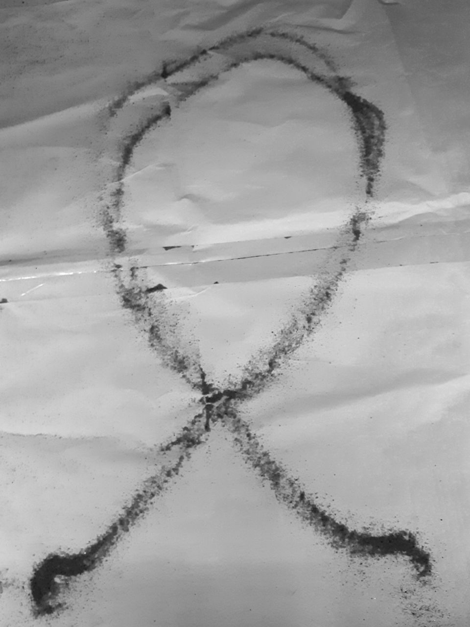
- 3D pendulum and imperfect figures:
It’s time to start swinging the actual 3d demo pendulum! The slides suggest starting with a 3/2 frequency ratio. This choice is mostly based on it giving a figure that is complex enough to be interesting without being too messy (if it has a lot of lines of sand a more precise swing is required).
The first swing done; it will naturally bring up the question of why it doesn’t look exactly like the figures from the Lissajous table. This is an opportunity to have students practice thinking like a scientist!
- Possible deviations from the ideal (a slide is included with illustrations of
some
phenomena):
- Air resistance – why do you have to keep pumping a swing at the playground, why don’t you swing forever? This is likely minimal though as the swing is short.
- Initial conditions/how you start the swing. This affects
- Phase
- Initial velocity (occasionally imparting a little rotational velocity)
- When the bob is supported by a hand rather than the string and then dropped, it and the bottle can sometimes act as a double pendulum, briefly oscillating relative to the string, and displaying a little chaotic behaviour in the beginning of the trajectory.
- Note that any mass lost from sand falling does not affect the trajectory as all the parameters are independent of mass. It could affect air resistance, but the heavy bob should ensure the affect is relatively small.
- Main demo:
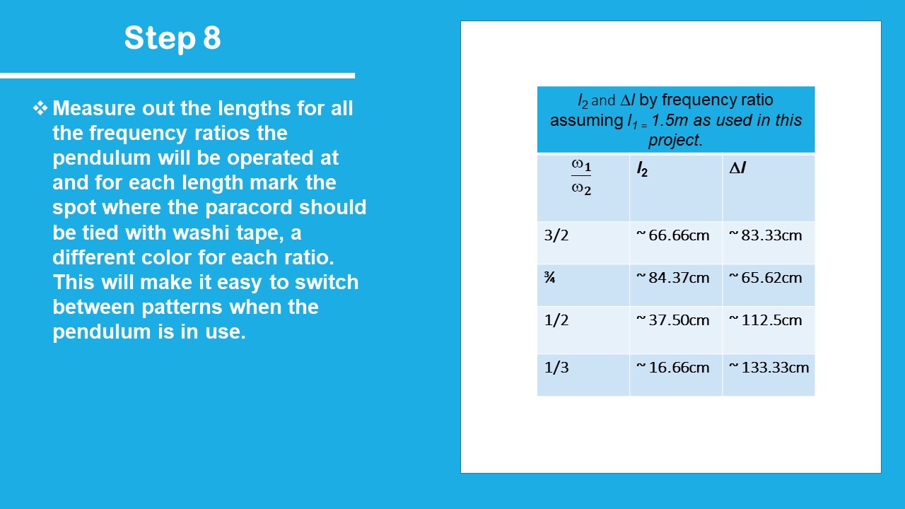
This section mostly consists of students playing with/experimenting with the 3d pendulum, but it is also where students will calculate the string lengths from periods (part 2 of the worksheet). A first calculation (the worksheet uses a ¾ ratio) and swing can be done together as a class and subsequent ones can follow as time allows.
Some concluding remarks can touch on:
- What are practical applications/ why is this problem interesting?
- The Lissajous machine revolutionized precision in music by allowing the calibration of tuning forks.
- Lissajous figures can be created with any oscillating waves, not just pendulums. Electro-magnetic Lissajous figures can be observed with an oscilloscope, for example.
- How physicists use concepts to think about real world solutions:
- Do you have any other harmonograph design ideas?
- The last slide shows some.
-2^(-4).jpg)