Materials & Equipment
- Light sensor
- Vernier LabPro interface
- Computer (laptop)
- Halogen light bulb
- Glass light diffuser
- Extension cord
- Motorized rotating table
- Power supply
- Ping-Pong ball
- Plastic ball (~4cm radius)
- 2 x ~30 cm stiff copper wire
- 2 x ~1.5m metal bars (one will have to be thick enough to support light source)
- 2 x clamps
- Base (for metal bars)
- Screw adjustable bosshead
- Clamp holder
- Black tablecloth
- Small stand
- Projector
- Projector (in classroom)
Arrangement
There will be two set-ups for the demo – one with the base, and one with the rotating table. The light source will be connected to the base for the first half such that it is easy to move around. And then for the second half about the transit method, the light source will be connected to the rotating table. In our case, the table was repurposed from a Coriolis effect demo.
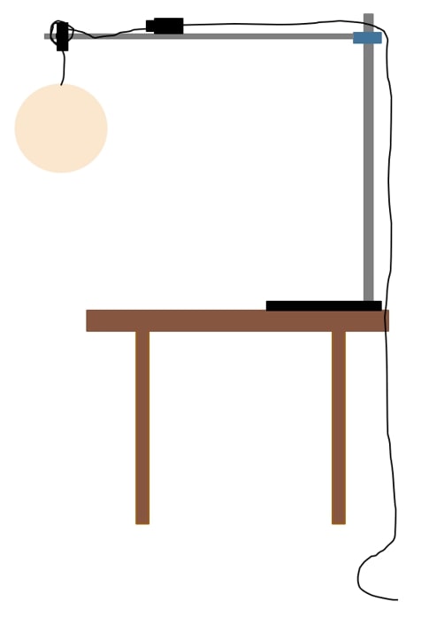
The light source that is connected to the base will consist if the two metal bars, one of the clamps, the bosshead, clamp holder, halogen light bulb, and the glass light diffuser. The metal bars will be connected using the clamp holder, and the bosshead will be placed on the thinner of the two bars. The halogen light bulb will be placed inside the light diffuser such that the luminosity is uniform on the diffuser’s surface. We will hang the light source by wrapping the wire around the bosshead and connecting it to the extension cord, which wire would run along the metal bar and then hang off the clamp holder. The set up with the base should look like this:
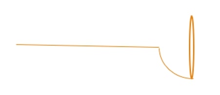
For the rotating table, a power source will be connected to the motor at the bottom of the table and will be placed at the opposite end of the table from the light sensor. The rotating table itself should be placed on a set of four tables put together into a square. The black cloth (which should have as little gloss as possible) will placed on the rotating table, over which the clamp will be placed, on the edge of the round, rotating part of the table. The copper wire will then be placed in the clamp, and the wire will itself be connected to either the ping-pong ball or the plastic ball. The copper wire will be bent such that it runs along a “longitudinal line” of the balls, and then bent such that it wraps around the ball along a “latitudinal line”. Tape will be placed on the first bent section to keep the ball in place, and this taped side will be placed such that it faces inward towards the light source. The wire would be bent somewhat like so:
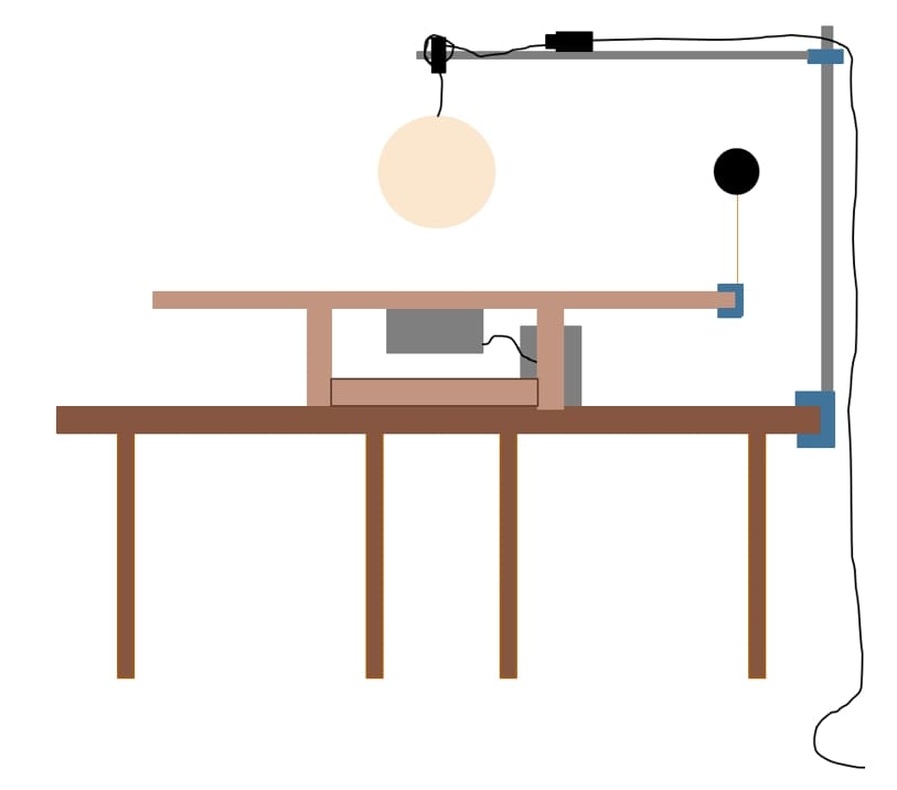
The ball will therefore rotate along with the table, with the copper wire blocking a small amount of light, but small enough compared to what either of the “planets” will block. Another clamp will be placed on one of the desks on which the rotating table is be standing on such that it is to the side of the table relative to the light sensor (not on the opposite side of the table from the light sensor). The light source will be placed on this clamp, and the set up with the light source should look like this:
As for the measurement side, the light sensor will be placed on a small stand on top of a desk a distance away from the light source, with a few more books or such placed below it so that it is level with the light source. The light sensor will be connected to the LabPro via one of its four channel ports. The LabPro will then be connected to the computer with double USB connection. The LoggerPro software will need to be installed to make used of the LabPro on the computer. Using this setup, we will be able to plot an intensity vs time graph in real time which will be projected for the students to see.